The economic determinants of forest clearing activity

21 July, 2011 - Dan Hammer

The Meridian Institute recently prepared a report for the Government of Norway on REDD+ reference levels. The primary authors are heavy hitters in the forest policy community, including Dan Zarin, Sandra Brown, and Arild Angelsen. They suggest that reference levels should be calibrated to reflect economic conditions -- that a simple, multi-year average rate is not sufficient for establishing a business-as-usual scenario. They do not specify, however, what those economic cofactors are, and how they affect forest clearing rates.

FORMA! One of the primary constraints in this field is the availability of data on forest clearing rates at high temporal resolution. FORMA was specifically designed to support research on the economic drivers of deforestation by providing monthly (and soon biweekly) updates on forest clearing activity in the humid tropics. We are writing a few papers that will be published soon (!) that link short-term deforestation rates with economic indicators, like real interest rates and the price of palm oil. Until then, I thought I'd post some code to estimate a spatial panel model.

Take, for example, the following generic system which describes a spatial error model with a spatial lag:

y = λWy + Xβ + u
u = ρWu + η

where y is a vector organized by panel group and date; X is a matrix of cofactors, also organized as a panel dataset; and W is a spatial weights matrix, which identifies panel units that are near each other. For administrative units, we define neighbors as units that share a common border. This generic system is described in Anselin (1988) via Millo and Piras (2009); and if ρ ≠ 0 and λ ≠ 0, then the model is subject to spatial dependence in both u (spatial error) and y (spatial lag). Ordinary least squares won't cut it. No, but thankfully Kapoor et al. (2007), among others, describe a maximum likelihood estimator for a spatially dependent panel -- which is implemented in R as part of the splm package. The code posted below reads in a standard dataset, admin_data.csv, alongside a shapefile of its administrative borders, admin_borders.shp, and then estimates a spatial error model with spatial lag.

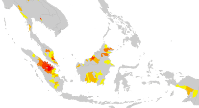
In our application, we found evidence that forest clearing activity does, in fact, respond to short-term economic indicators. A few variables that survived multiple rounds of shock testing were cell phone coverage, palm oil futures, and real interest rates -- all lagged by 6-18 months. A cool, compact result is that λ tends to be large and significant -- somewhere in the 0.4-0.6 range. This implies (to an extent) that forest clearing will be clustered, which is apparent from just looking at the maps. Check out the map below, which highlights subprovinces with particularly high forest clearing rates in Southeast Asia between 2000 and 2005. [Yellow to red indicates more intense clearing rates within the subset of subprovinces with high clearing rates.] There is definitely some spatial inertia associated with deforestation. Clusters of deforestation tend to bloom like an infectious disease; and these clusters, in turn, tend to be clustered.

Running the estimation is not a trivial. Our panel is comprised of 193 subprovinces, each with 60 observations (5 years at monthly intervals). To properly test the robustness of the results, we ran many, many iterations of the model, searching for the one that was most likely, given the data. For this, we used Amazon.com's cloud computation platform. We employed our own cluster to churn through different specifications. We wrote the entire cluster and queue management system in Python. I'll post some code soon.

## Basic R script to estimate a spatial panel model
## Install packages, if necessary
install.packages(c("maptools", "splm", "spdep"))

## Load packages
library(maptools)
library(splm)
library(spdep)

## Read in the CSV and shapefile data.  Be sure that the files
## admin_borders.dbf and admin_borders.prj are stored alongside
## admin_borders.shp in the same folder.  Note that the function
## readShapePoly() requires only the file name, without an extension.
## Note also that the two leftmost variables of admin_borders.csv
## should be panel group ID and date, if you do not use a panel data
## frame (look up pdata.frame).
data <- data.frame(read.csv("admin_data.csv"))
xx <- readShapePoly("admin_borders")

## Create spatial weights matrix.  The snap parameter for polygons
## will identify a neighboring area, even if the borders are not 
## adjacent, but within 0.1 spatial units (arcdegrees in this case.).
## The style "W" will row-standardize the weighting matrix so that
## each row sums to 1.  zero.policy will allow for areal units with
## no links.  fm is the model that you want to estimate.
Wmat <- nb2listw(poly2nb(xx, snap=.1), style = "W", zero.policy=TRUE)
fm <- y ~ X

## Spatial error model with spatial lag, based on Kapoor, et al. (2007)
spml.res <- spml(fm, data=data, listw=Wmat, 
                     model="random", lag=TRUE, spatial.error="kkp")
(summary(spml.res))

The economic determinants of forest clearing activity

Related Posts